Damage And Loss Assessment Due To Tropical
Cyclone Idai’s Flooding Events In Chimanimani District
Rumbidzai Chivizhe, Juliana Useya, Reason Mlambo,
Zimbabwe
This article in .pdf-format
(16 pages)
1. INTRODUCTION
Natural disasters are calamities with atmospheric, geological, and
hydrological causes that have the potential to result in casualties,
property destruction, and social and environmental disturbance (Xu et
al., 2016). Examples of these natural disasters are, droughts,
earthquakes, floods, cyclones and landslides. The most destructive
natural disasters are tropical cyclones, which usually pose a
significant danger of human fatalities, significant financial loss, and
significant environmental damage (Charrua et al., 2021). Some of the
tropical cyclones experienced in Zimbabwe included Cyclone Eloise,
Tropical Storm Ana, and Cyclone Jasmine, causing significant damage in
Zimbabwe (Mukwenha, 2021). In Zimbabwe, the disaster that was
experienced in March 2019 was tropical cyclone Idai which was
accompanied by flash floods, lightning, hail, and heavy rains. As a
result of the catastrophic effects on agriculture, schools, and
infrastructure, many residents lost their houses, infrastructural loss,
casualties and disruption of daily life (Chatiza, 2019). Fluvial
flooding was experienced in Chimanimani district and can be classified
into two primary categories: overbank flooding and flash flooding. Flash
flooding is defined as a fierce torrent of water over an
already-existing river at a fast rate of speed. Flood extent may now be
successfully mapped thanks to current technology, such as geographic
information systems and remote sensing (Ward et al. 2014; Ho et al.
2010; Samarasinghea et al. 2010).
In this research, the cyclone Idai flood damage and loss assessment
was done using both SAR data and optical data; nonetheless, microwave
(SAR) satellite data is a more preferable method for flood mapping
because it has the ability to capture images day or night regardless of
weather conditions (Anusha & Bharathi, 2020). Damage and loss assessment
are imperative for flood management although it is a challenging task
due to its complexity in dealing with big data, damage types, spatial
and temporal scales i.e. depth of analysis (Menoni et al., 2016). GIS
and remote sensing, often known as Earth Observation System (EOS), are
nowadays the most used tools for disaster management (Simonovic & Eng,
2002). The actual flood extent cannot be assessed fully from field
visits because of the area vastness and the restriction of mobility,
thus EO data is important (Husain & Shan, 2010). This is because it
gives an advantage where data is limited, costly and hard to access and
needs frequent revisit times (Clement et al., 2017). Satellite data are
crucial for identifying, assessing, and quantifying flood extent,
damage, and environmental effects, according to several authors
(Hussaina et al. 2011; Khanna et al. 2006). Optical and radar data is
common for flood monitoring and damage assessment and proven to be
efficient in flood inundation mapping because of their distinct
properties. The optical data’s distinct water reflectance property makes
it effective in identifying water bodies from other land uses as it is
displayed in terms of the spectral bands (Husain & Shan, 2010). This
property helps to efficiently delineate vegetation from other land
covers using a near-infrared and red band optical imagery. Synthetic
aperture radar (SAR) sensors’ microwave capabilities of being able to
penetrate through clouds and its applicability for both day and night
makes it extremely good for flood water extraction (Jussi, 2015;
Schlaffer et al, 2015). The optical and radar data sets are finally
combined through feature level fusion in order to bring out the desired
outcome. The radar datasets in this study came from the Sentinel-1
databases, whereas the optical datasets come from Sentinel-2. In this
investigation, feature level fusion was used to combine optical and
radar data. When two or more images are combined to create a composite
image, the information from each individual image is integrated, giving
the finished image a higher information content than any of the input
images. "Image fusion" is the name of this procedure (Pradham et al.,
2010). Finding a transformation of the original space that would produce
these new features, which are conserved or improved to the greatest
extent possible, is the aim of feature level fusion.
In terms of Zimbabwe’s context, some authors only determined the
Cyclone Idai’s flood extent while others estimated the general damage
and losses that came as a result of the cyclone which did not clearly
bring out the exact damage and loss that came as a result of flooding.
As a result, the main research gap in the current study is the
inadequacy of knowledge regarding the amount of damage and loss that
resulted from the cyclone’s flood in Zimbabwe’s Chimanimani district.
Therefore, the objectives of this research are to (i) spatially
explicitly map the flooded area extent, (ii)evaluation of the effects of
flood brought on by cyclone Idai through moderate spatial resolution
imagery (Radar and Optical) and (iii) determining the amount of damage
and loss brought on by cyclone Idai’s flooding events as per land-use
class. The novelty of this study was on using radar in mapping flood
extents and then fusing through feature level fusion, with optical data
considering spectral indices, thus, NDVI and NDBI. Change detection
based on the NDVI and NDBI spectral index on the inundated area is
conducted with the intention to determine damage and loss within the
study area.
2. study Area
2.1 Study Area: Chimanimani District
A mountainous district in the Manicaland Province of south-eastern
Zimbabwe is the Chimanimani District. The town of Chimanimani also
serves as the district capital. It covers an area size of 3,450.14 km2.
Its borders are as follows: Mozambique to the east, Mutare District to
the north and northwest, Buhera District to the west, and Chipinge
District to the south. The eastern portion of the district is bordered
by the Chimanimani Mountains, which run for about 50 kilometers (31
miles) and constitute the border with Mozambique. From September 5 to
July 20 of each year, Chimanimani experiences 10 months of rain, with a
typical 31-day rainfall of at least 0.5 inches. The wettest month is
January, with an average rainfall of 7.6 inches, while the driest is
August, with an average rainfall of 0.3 inches. Hence, the rainless
period of the year lasts for 1.5 months (weatherspark.com). However,
rainfall typically consists of powerful thunderstorms and is caused by
low pressure systems travelling north-east up the Mozambique channel and
inland. Rainfall rises sharply with altitude, reaching 2000mm at higher
altitudes from roughly 1200mm annually along south-east-facing foothills
(CNR Management Plan, 2010). The majority of the soils in Chimanimani
district are white sands, which have a very limited capacity to retain
water and low fertility (BirdLife International, 2023).
3. Materials
3.1 Satellite data
3.1.1 Sentinel 1 (SAR/Radar)
For this work, Sentinel-1 Ground Range Detected (GRD) single
co-polarized imagery was used to map the flood extent in the study area.
It was downloaded from Copernicus Open Access Hub,
Link.
3.1.2 Sentinel-2 (Optical)
This study uses Sentinel-2 imagery to evaluate flood damage in the
study area. The Copernicus Open Access Hub was used to get the data from
the Sentinel-2 SAR satellite operated by the European Space Agency. With
spatial resolutions between 10m and 20m, each MSI contains 13 spectral
bands that encompass the visible, red-edge, near-infrared (NIR), and
short-wave infrared (SWIR) wave lengths. Both the sentinel-1 and
sentinel-2 data collected are displayed in Table 1.1 below.
| Satellite |
Acquisition date before floods |
Acquisition date after floods |
| Sentinel-1 |
07 March 2019 |
19 March 2019 |
| Sentinel-2 |
28 February 2019 |
25 March 2019 |
4. Methodology
4.1 Methodology for Radar
The subset of the image, multilooking, radiometric calibration is
part of the pre-processing for Sentinel-1's synthetic aperture radar
(SAR) data using the Sentinel Snap software. Geometric and radiometric
distortion occur as a result of SAR's ability to see the topography from
the side. The geometry has been rebuilt using a DEM and is prepared for
geometric correction of terrain distortions (Akbari et al., 2012). A
digital elevation model (1 Arc Sec SRTM DEM) is used for terrain
correction in SAR geocode images to correct for geometric errors and
provide a map-projected result. The DEM was downloaded independently for
this investigation from USGS Earth Explorer. The data were reprojected
using range doppler terrain correction with WGS84. Layer stacking is
used to combine the before and after flood images using the VV
polarization because it can identify partially submerged features that
help assess flood damage (Rao et al., 2006). The bands from both scenes
are combined in the stacked image, therefore in this case, the red band
from the before flood and the red and blue bands from the after-flood
band were utilized to form the RGB composite. The final image, which was
used to produce a flood map as a geotiff which depicts the flood extent.
To evaluate the flood damage, the Sentinel-2 NDVI and NDBI scenes will
be merged with the flood extent map.
4.2 Methodology for Optical
The Sentinel-2 images that were collected from Copernicus Hub, for
this study were on Level 2A and had already undergone radiometric and
geometric correction. The atmospheric adjustment was then performed
using Sen2Cor by translating the Sentinel-2 Top of Atmospheric
Reflectance into the appropriate Bottom of Atmospheric adjusted Level 2A
products.
4.2.1 Normalized Difference Vegetation Index (NDVI)
NDVI was employed in this work to track changes in plant cover using
the downloaded Sentinel-2 data. An indicator of vegetation greenness
used in remote sensing, the Normalized Difference Vegetation Index
(NDVI), is linked to the structural characteristics of plants. NDVI time
series can be used to analyze the majority of vegetation changes (Forkel
et al, 2013). The visible and near infrared portions of the
electromagnetic spectrum are used by the NDVI. This is due to the fact
that vegetation, such as forests, exhibits substantial absorption in the
red area (0.63-0.69u m) and increased reflectance in the near IR range
(0.76-0.90u m). The distribution of vegetation is specifically defined
by this ratio. The following formula is used to determine NDVI values:
NDVI= (NIR-RED/NIR+RED) The NDVI readings are displayed as a ratio from
-1 to +1, with the majority of the (-) values denoting water and the
rest values falling within the negatives denoting soil/built-up. The
categorization considered the variation in NDVI values before and after
floods and decided that positive values indicated the presence of
vegetation, while negative values indicated that there was no vegetation
present and were represented as No Data values.
4.2.2 Normalized
Difference Built-up Index (NDBI)
In this study, built-up cover change was tracked using NDBI and the
downloaded Sentinel-2 data stated above. The NDBI, which has indices
ranging from -1 to 1, is one of the spectral indices designed
specifically for extracting man-made surfaces. The electromagnetic
spectrum's shortwave-infrared and near-infrared frequencies are used by
the NDBI. The following formula is used to determine NDBI values: NDBI=
(SWIR-NIR)/(SWIR+NIR). The NDBI values are displayed as a ratio between
-1 and +1; the majority of the (-) values correspond to water, while the
other numbers within the negatives correspond to vegetation. The
categorization considered the variation in NDBI values between before
and after floods and decided that positive values indicated the presence
of built-up, while negative values indicated the absence of built-up and
were represented as No Data values.
4.4. Fusion of Optical and
Synthetic Aperture Radar (SAR) data
The generated NDVI and NDBI Difference results were fused using
feature level fusion with the vectorized flood extent to extract only
the NDVI flooded area and the NDBI flooded area in order to determine
both the positive and negative change. The outcome was divided into
three categories—decrease, no change, and increase—which clearly
demonstrated the amount of the harm. The raster layer unique values
report tool was used to collect the statistical values in respect to the
decline, no change, and increase class in terms of hectarage.
The
flowchart of the methodology in this study area is shown in Figure 2.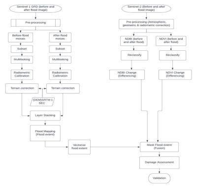
Figure 2. Flowchart for the workflow
5. Results and Discussion
5.1 Flood Extent mapping
Sentinel-1 images of the pre- and post-flood events were collected to
determine the extent of the flooding episodes under study (Table 1).
Water features are distinguished from other features after
pre-processing both images using sigma nought (0) distribution as the
backscatter coefficient. These backscatter values show the non-water
class as higher values and the water class as lower values (Lurist et
al., 2017). After thresholding, the research area's water class is
generated. After that, the images were combined by building a layer
stack with the help of the product's geolocation. The investigation
region's water class is generated when the edge is joined. To
discriminate between the flooded areas and the permanent water bodies,
an RGB composite image is produced. The pre-flood image fills the red
band for this, and the post-flood image fills the blue and green bands.
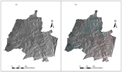
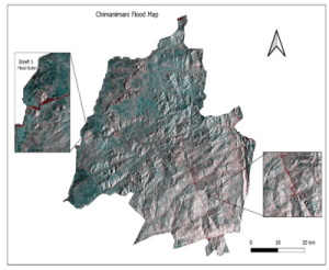
Figure 5. Showing Chimanimani (a) Pre-flood period, with dark
gray color representing the river channel and (b) Post-flood period,
with the red color representing the flooded river channel.
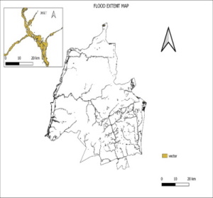
Figure
6a. Chimanimani area tropical cyclone flood map. Figure 6b. Vectorized
flood extent map.
This is done such that the flooded areas on the red
channel will have a high radar response because they will land on the
pre-flood image, leading to a high backscatter return. However, on the
post-flood image, the flooded areas will have a low backscatter return.
The purpose of this is to make the flooded areas appear in red because
they will have high red channel response and low blue and green channel
response, while the surrounding areas where there is no flood appear as
tones of grey with a bluish color because they have low backscatter
return in both images, which means low response in all the red, green,
and blue bands. To determine the extent of flooding caused by the
cyclone, water features of the flooding were mapped, and the results
were compared with permanent water bodies. The flooded area in
comparison to non-flooded area is shown on Figure 5 whilst the
Chimanimani flood map is clearly depicted in Figure 6a.The flooded areas
are then vectorized by exporting the map of the affected area as a
geotiff; the vector map is depicted in figure 6b.
The red tones
symbolize flood surfaces where the water has totally flooded, while the
light pink tones are typical of humid environments. The distinction of
flooded areas is best when the polarization is chosen correctly (Klemas,
2015). The findings from our polarization configurations and the
contributions from studies comparing polarizations to monitor flood
zones confirm that the VV polarization is more effective at delimiting
flooded areas (Martinis & Rieke, 2015). It creates well-defined surfaces
with the ability to identify partially submerged features, providing
data that VH polarization may not be able to provide because it is
predicated on the terrain's heterogeneity and roughness (Manjusree et
al., 2012).
The validation of the flood extent was carried out by
extracting the extent of the flood using NDWI, which produced results
that were identical, particularly with regard to the flooding in rivers
and permanent water bodies. The same SAR method was tested in order to
map the flood extent in Mozambique, and it was successful in doing so.
5.2.1 Impacts of flood on Vegetation using NDVI
NDVI values range from -1 to +1, the non-vegetation class is
eliminated from the analysis by reclassifying before and after flood
images. Figure 8 shows the NDVI before and after flood map. On the basis
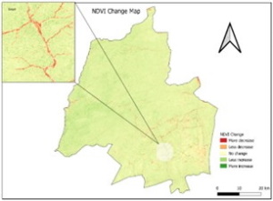
of the classified image, NDVI Difference is then determined and the
results of the change detection are presented on Figure 9. The five
classes used to depict the NDVI Differencing results above are more
increase, less increase, no change, less decline, and more decrease.
Although the flooded areas exhibit the complete opposite, the data
indicate that there are often more locations with vegetation that has
somewhat increased than those shown by the "less increase" class. The
places with a greater loss of vegetation, in particular, are depicted as
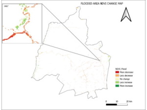
having vegetation inside of flooded areas. The sentinel-1 resultant
vectorized image showing the flood extent is merged with the Sentinel-2
NDVI change image. This gives us the flooded area NDVI change layer as
shown in Figure 10 below.
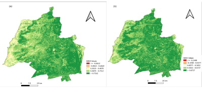
Figure 8. Showing (a) NDVI Pre-flood period and (b) NDVI Post flood
period.
The change detection statistics are calculated based on the
extracted flooded NDVI change area with reference to the changes
represented in the figure above. The more decrease and less decrease are
classified as negative change, the less increase and more increase as
positive change while no change remains the same. The results are shown
in Table 2.
 |
 |
| (a) |
(b) |
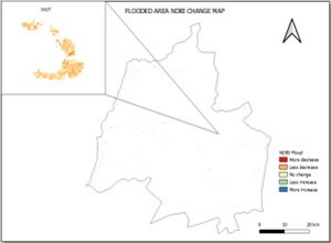
Figure 9 (a) Shows the NDVI Change Detection for cyclone Idai flooding
event and Figure 9 (b). showing the flooded area NDVI change scenes.
Table 2. Change detection statistics for vegeta
| Class |
Area |
% Change |
| Postive Change |
236,57 Ha |
5.98 |
| No Change |
4.33 Ha |
0.11 |
| Negative Change |
3716 Ha |
93.91 |
According to the table, the class of depleted vegetation is exhibiting
the highest change, with a change of 93.91 percent, compared to
vegetation that saw no change as a result of flooding, with a change of
0.11 percent. The 5.98 percent margin represents the vegetation that
changed more than average. The estimation of the damage and loss
experienced in terms of vegetation is 93.91% which corresponds to 3716Ha
of negative change. This means then that almost all the vegetation that
was mainly along the river beds was damaged by the flash floods
experienced during cyclone Idai among other flooded areas. The no change
and positive change representing no damage, corresponds to some
vegetation that adapts to flood such as a number of tress like acacia
and mopane and some rice plants which flourish with too much water
present.
5.2.2 Impacts of flood on built-up areas using NDBI
There was a need to exclude the non-built up areas from the differencing
process, hence any feature which corresponded to non-built up was
assigned no data value. The image that results is utilized to determine
the NDBI Difference. Figure 8 below shows the results of the change
detection calculations for the Cyclone Idai flood occurrences.
 |
 |
| (a) |
(b) |
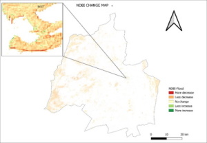
Figure 12a. Showing NDBI change and Figure 12b. Showing the flooded area
NDBI change scenes
The figure 12a above shows the NDBI change for periods between before
and after flood. The results indicate that, there has been a significant
decline in built-up, no change regions and a less pronounced increase in
built up areas. The sentinel-1 resultant vectorized image showing the
flood extent is merged with the sentinel-2 NDBI change image. This gives
us the flooded area NDBI change layer as shown in Figure 12b. The
following table was created with reference to changes that have taken
place since the cyclone Idai flood event using the change detection
statistics in QGIS. The no change class stays the same while the more
decrease and less decrease classes are combined to form the negative
change class and the more increase and less increase classes are
combined to form the positive change class. The findings of the change
detection are shown in Table 3 below in three groups for positive
change, no change, and negative change.
Table 3. Change detection statistics for built-up areas
| Class |
Area |
% Change |
| Postive change |
233.60 Ha |
20.56 |
| No change |
581,58 Ha |
51.19 |
| Negative change |
320.98 Ha |
28.25 |
The findings from this study, demonstrate that indeed floods have an
effect on built-up areas. The positive change in built-up areas, of
hectarage as 233.60Ha, giving us an estimate of 20.56 percent. This
damage presented by 28.25 percent is explained by the houses, bridges
and roads that were swept away by water. No change which has a highest
representation of 51.19 percent, shows us that vast areas which were
made up of infrastructure were not affected by flood, hence the
structures are still intact. The positive change however, could mean
those buildings that were immediately erected after flood for
resettlement and also a few drawbacks of using NDBI such as noise due to
some barren ground particularly uncultivated arable land which may have
similar spectral response patterns. According to the Government of
Zimbabwe data by Chatiza (2019), 61.5% of dwellings in Chimanimani were
damaged. Since a variety of elements, such as landslides, wind, stones
falling, and water, contributed to the damage to homes in Chimanimani.
We therefore conclude that 28.25% of the 61.5 % of damaged dwellings in
Chimanimani were caused by flood.
6. Analysis of Results
The storm left a path of destruction causing the deaths of people as
well as significant damage to crops, livestock, and property. Road
infrastructure was grossly damaged with above 90% of road networks in
Chimanimani and Chipinge damaged and 584 km of roads being damaged by
landslides. Bridges were also swept away. The shortage of fit for human
habitation land has forced some people to settle along waterways that
are prone to landslides and there is also apparent stream bank farming
around many rivers and river sources (Munsaka et al, 2021). The building
materials commonly used for construction of walls and roof of houses in
rural areas are clay, sand, bamboo, grass, reeds, timber and stone.
These can be easily washed away by floods especially if built along
waterways. On the other hand, bridges and roads which also fall under
the category of built-up areas were constructed using steel, concrete,
stone and asphalt, had several of them washed away by the flood due to
the pressure caused by the flood. There is also an issue of degraded
land observed in soil compaction, increased run-off, loss of soil
fertility, and decrease in vegetation cover which cause low river
volumes thus increasing the vulnerability to flooding and landslides
(Munsaka et al, 2021). According to assessment by the Environmental
Management Agency (EMA) in 2009, areas affected by water were mainly
located in floodplains, along waterways and on steep slopes. This was
evident as presented on the flood map on figure 6 which shows that flood
was mostly along the river course. Extreme seasonal changes in monthly
rainfall occur in Chimanimani, which accounts for cyclone Idai's
appearance in March 2019 as one of the anomalies. People in Chimanimani
district have most of their planting and irrigation close to the rivers,
these are plants such as bananas, yam, maize and some tea estates were
negatively damaged by the floods. There was also a case of insects which
came as a result of the flood that destroyed a certain maize field.
According to my research, of the total area of Chimanimani district
which is 3,450.15km2, about 5882.32Ha was submerged under water during
cyclone.
7. Conclusion
The study’s main objective was to evaluate the damage and loss which
came as a result of flooding in Chimanimani district due to tropical
cyclone Idai in March 2019. This was achieved by using Sentinel-1 SAR
data to map the flood extent and Sentinel-2 data to determine the
vegetation and built-up affected by flood. For analysis, this was later
combined through feature level fusion to determine the damage and loss
on the flooded areas only. A lot of vegetation was affected by cyclone
Idai compared to the infrastructure that was destroyed by the cyclone.
The rehabilitation efforts, as explained before, should target first
those inhabitants along waterways and on floodplains as they were the
most affected by floods. Particularly vulnerable to flooding were the
Ngangu, Kopa, and other residential areas, which were exposed more than
other regions (Munsaka et al, 2021). A key factor in lessening a
community's vulnerability to disasters is the town planners and local
institutions' ability to do their duties. The capacity of communities to
prepare for and respond to flooding is increased by climate risks
education and awareness. This research is unique in that it has
distinguished between the loss and damage brought on by Cyclone Idai’s
flooding events compared to those that considered it in general. There
were however, limitations due to the image’s resolution which made it
difficult to assess damage per each vegetation type and built-up class
in particular which I would recommend the other researchers to further
the study by focusing on the specifics given higher resolution imagery.
References
- Akbari, V., Larsen, Y., Doulgeris, A. P., & Eltoft, T., 2012.
The impact of terrain correction of polarimetric SAR data on glacier
change detection. In International Geoscience and Remote Sensing
Symposium (IGRASS), pp. 5129-5132.
- Anusha, N., & Bharathi. V., 2019, Flood detection and flood
mapping using multi-temporal synthetic aperture radar and optical
data. The Egyptian Journal of Remote Sensing and Space Science. 23.
- Arun, R. & Premalatha, K., 2020. Flood Damage Assessment Using
Remote Sensing and GIS: The Past and Present. International Journal
of Civil Engineering and Technology (IJCIET), 11(12), pp. 1-15.
- BirdLife International, 2023, BirdLife International’s Position
on Climate Change. Cambridge, Uk.
- Charrua, A. B., 2021, Impacts of the Tropical Cyclone Idai in
Mozambique: A Multi-Temporal Landsat Satellite Imagery Analysis.
Remote Sensing, 13(201).
- Chatiza, K., 2019. Cyclone Idai in Zimbabwe. An analysis of
policy implications for post-disaster ins disaster risk management,
p. 2.
- Clement, M. A., Kilsby, C. G. & Moore, P., 2017, Multi-temporal
synthetic aperture radar flood mapping using change detection.
Journal of Flood Risk Management, pp. 0-17.
- CNR Management Plan, 2010, Agro Ecological Regions and Climate
of Chimanimani, Appendix2
- Forkel, M., Carvalhais, N., Verbesselt, J., Mahecha, M. D.,
Neigh, C. S., & Reichstein, M., 2013, Trend change detection in NDVI
time series: Effects of inter-annual variability and methodology.
Remote Sensing. 5(5), 2113-2144.
- Hussaina, E., Urala, S., Malikb, A. & Shana, J., 2011, Mapping
Pakistan 2010 floods using remote sensing data: ASPRS Annual
Conference. Milwaukee, WI, USA, s.n.
- Hussain, E. & Shan, J., 2010, Mapping major floods with optical
and sar satellite images. IEEE Geoscience and Remote Sensing
Symposium, Honolulu, Hawaii, USA, (July), pp. 25-30.
- International Federation of Red Cross and Red Crescent
Societies, 2019, Zimbabwe: Tropical Cyclone Idai, s.1: International
Federation of Red Cross and Red Crescent Societies
- Jussi, M., 2015, Synthetic Aperture Radar based flood mapping in
the Alam-Pedja Nature Reserve in years 2005-2011.
- Klemas, V., 2015, Remote sensing of floods and flood-prone
areas. An Overview. J. Coast. Res. 31, pp. 1005-1013.
- Lurist, N., Lurist, N.V., Oniga, V.E., Statescu, F. and Marcu,
C., 2012, Floods damage estimation using Sentinel-1 satellite
images. Case study-GALATI COUNTY, ROMANIA.
- Martinis, S. & Rieke, C., 2015, Backscatter analysis using
multi-temporal and multi-frequency SAR data in the context of flood
mapping at river Saale, Germany. Remote Sensing, 7, pp. 7732-7752.
- Menoni, S., Molinari, D., Ballio, F., Minucci, G., Mejri, O.,
Atun, F., Berni, N., and Pandolfo, C., 2016, Flood damage: a model
for consistent, complete and multipurpose scenarios, Nat. Hazards
Earth Syst. Sci., 16, 2783–2797
- Mukwenha S, 2021. Health emergency and disaster risk management:
A case of Zimbabwe's preparedness and response to cyclones and
storms: We are not there yet, Harare: Public Health in Practice.
- Munsaka, E., Mudavanhu, C., Sakala, L., Manjeru, P., Matsvange,
D., 2021, When Disaster Risk Management Systems Fail: The Case of
Cyclone Idai in Chimanimani District, Zimbabwe. International
Journal of Disaster Risk Science, 12, pp. 689-699.
- Pradhan, B.,2010, Flood susceptible mapping and risk area
delineation using logistic regression, GIS and remote sensing. J
Spatial Hydrol 9:1–18
- Rao, G. S., Brinda, V., Sree, P. M., & Bhanumurthy, V. 2006,
Advantage of Multi-polarized SAR data for Flood Extent Delineation.
64100.
- Schlaffer, S., Matgen, P., Hollaus, M. & Wagner, W., 2015, Flood
detection from multi-temporal SAR data using harmonic analysis and
change detection. International Journal of Applied Earth Observation
and Geoinformation, Volume 38, pp. 15-24.
- Simonovic, S. P. & Eng, P., 2002, Role of remote sensing in
disaster management, s.l.: s.n.
- Ward, D. et al., 2014. Floodplain inundation and vegetation
dynamics in the Alligator rivers region (kakadu) of northern
Australia assessed using optical and Radar Remote Sensing. Remote
Sensing of Environment,147, pp. 43-55.
https://doi.org/10.1016/j.rse.2014.02.009
- Xu, J., Wang Zi., Shen, F., Ouyang, C., Tu, Y., 2016, Natural
disasters and social conflict: A systematic literature review,
International Journal of Disaster Risk Reduction,17, pp. 38-48.
BIOGRAPHICAL NOTES
(Corresponding author)
Rumbidzai Chivizhe
2012-2017 Bsc Honors Degree Surveying and Geomatics (Midlands State
University)
2017-2022 Land Surveyor in Training (D. Chigumbu Land Surveyors-
Zimbabwe)
2021-2023 Honorary Treasurer (Survey Institute of Zimbabwe) 2021-2022
Msc Geomatics Engineering (University of Zimbabwe)
CONTACTS
Mrs Rumbidzai Chivizhe
Survey Institute of Zimbabwe
Suite4, Phyllis Court, 3
Raleigh Street,
Harare,
Zimbabwe